tbl_svysummary: Create a table of summary statistics from a survey object

Description

The tbl_svysummary function calculates descriptive statistics for continuous, categorical, and dichotomous variables taking into account survey weights and design. It is similar to tbl_summary().

Usage

tbl_svysummary(
  data,
  by = NULL,
  label = NULL,
  statistic = NULL,
  digits = NULL,
  type = NULL,
  value = NULL,
  missing = NULL,
  missing_text = NULL,
  sort = NULL,
  percent = NULL,
  include = everything()
)

Value

A tbl_svysummary object

Arguments

data: A survey object created with created with survey::svydesign()
by: A column name (quoted or unquoted) in data. Summary statistics will be calculated separately for each level of the by variable (e.g. by = trt). If NULL, summary statistics are calculated using all observations. To stratify a table by two or more variables, use tbl_strata()
label: List of formulas specifying variables labels, e.g. list(age ~ "Age", stage ~ "Path T Stage"). If a variable's label is not specified here, the label attribute (attr(data$age, "label")) is used. If attribute label is NULL, the variable name will be used.
statistic: List of formulas specifying types of summary statistics to display for each variable. The default is list(all_continuous() ~ "{median} ({p25}, {p75})", all_categorical() ~ "{n} ({p}%)"). See below for details.
digits: List of formulas specifying the number of decimal places to round summary statistics. If not specified, tbl_summary guesses an appropriate number of decimals to round statistics. When multiple statistics are displayed for a single variable, supply a vector rather than an integer. For example, if the statistic being calculated is "{mean} ({sd})" and you want the mean rounded to 1 decimal place, and the SD to 2 use digits = list(age ~ c(1, 2)). User may also pass a styling function: digits = age ~ style_sigfig
type: List of formulas specifying variable types. Accepted values are c("continuous", "continuous2", "categorical", "dichotomous"), e.g. type = list(age ~ "continuous", female ~ "dichotomous"). If type not specified for a variable, the function will default to an appropriate summary type. See below for details.
value: List of formulas specifying the value to display for dichotomous variables. gtsummary selectors, e.g. all_dichotomous(), cannot be used with this argument. See below for details.
missing: Indicates whether to include counts of NA values in the table. Allowed values are "no" (never display NA values), "ifany" (only display if any NA values), and "always" (includes NA count row for all variables). Default is "ifany".
missing_text: String to display for count of missing observations. Default is "Unknown".
sort: List of formulas specifying the type of sorting to perform for categorical data. Options are frequency where results are sorted in descending order of frequency and alphanumeric, e.g. sort = list(everything() ~ "frequency")
percent: Indicates the type of percentage to return. Must be one of "column", "row", or "cell". Default is "column".
include: variables to include in the summary table. Default is everything()

statistic argument

The statistic argument specifies the statistics presented in the table. The input is a list of formulas that specify the statistics to report. For example, statistic = list(age ~ "{mean} ({sd})") would report the mean and standard deviation for age; statistic = list(all_continuous() ~ "{mean} ({sd})") would report the mean and standard deviation for all continuous variables. A statistic name that appears between curly brackets will be replaced with the numeric statistic (see glue::glue).

For categorical variables the following statistics are available to display.

{n} frequency
{N} denominator, or cohort size
{p} percentage
{p.std.error} standard error of the sample proportion computed with survey::svymean()
{n_unweighted} unweighted frequency
{N_unweighted} unweighted denominator
{p_unweighted} unweighted formatted percentage

For continuous variables the following statistics are available to display.

{median} median
{mean} mean
{mean.std.error} standard error of the sample mean computed with survey::svymean()
{sd} standard deviation
{var} variance
{min} minimum
{max} maximum
{p##} any integer percentile, where ## is an integer from 0 to 100
{sum} sum

Unlike tbl_summary(), it is not possible to pass a custom function.

For both categorical and continuous variables, statistics on the number of missing and non-missing observations and their proportions are available to display.

{N_obs} total number of observations
{N_miss} number of missing observations
{N_nonmiss} number of non-missing observations
{p_miss} percentage of observations missing
{p_nonmiss} percentage of observations not missing
{N_obs_unweighted} unweighted total number of observations
{N_miss_unweighted} unweighted number of missing observations
{N_nonmiss_unweighted} unweighted number of non-missing observations
{p_miss_unweighted} unweighted percentage of observations missing
{p_nonmiss_unweighted} unweighted percentage of observations not missing

Note that for categorical variables, {N_obs}, {N_miss} and {N_nonmiss} refer to the total number, number missing and number non missing observations in the denominator, not at each level of the categorical variable.

Example Output

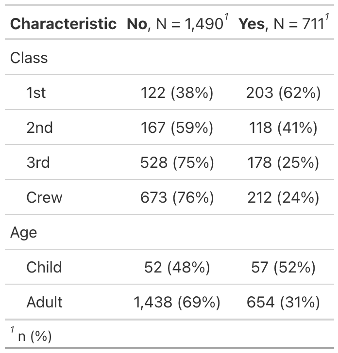
Example 1

image of rendered example table

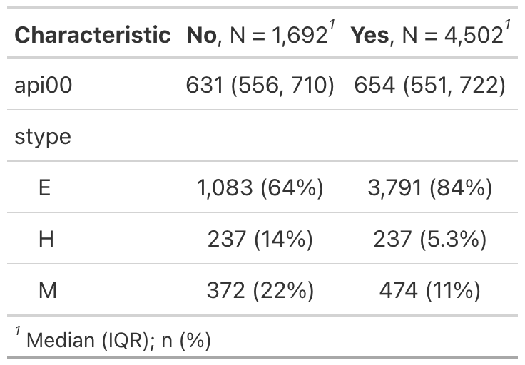
Example 2

image of rendered example table

type argument

The tbl_summary() function has four summary types:

"continuous" summaries are shown on a single row. Most numeric variables default to summary type continuous.
"continuous2" summaries are shown on 2 or more rows
"categorical" multi-line summaries of nominal data. Character variables, factor variables, and numeric variables with fewer than 10 unique levels default to type categorical. To change a numeric variable to continuous that defaulted to categorical, use type = list(varname ~ "continuous")
"dichotomous" categorical variables that are displayed on a single row, rather than one row per level of the variable. Variables coded as TRUE/FALSE, 0/1, or yes/no are assumed to be dichotomous, and the TRUE, 1, and yes rows are displayed. Otherwise, the value to display must be specified in the value argument, e.g. value = list(varname ~ "level to show")

select helpers

Select helpers from the \tidyselect\ package and \gtsummary\ package are available to modify default behavior for groups of variables. For example, by default continuous variables are reported with the median and IQR. To change all continuous variables to mean and standard deviation use statistic = list(all_continuous() ~ "{mean} ({sd})").

All columns with class logical are displayed as dichotomous variables showing the proportion of events that are TRUE on a single row. To show both rows (i.e. a row for TRUE and a row for FALSE) use type = list(where(is.logical) ~ "categorical").

The select helpers are available for use in any argument that accepts a list of formulas (e.g. statistic, type, digits, value, sort, etc.)

Read more on the syntax used through the package.

Author

Joseph Larmarange